CS280A Project 5: Fun With Diffusion Models!

Part A: The Power of Diffusion Models!

Part A.0: Setup

In the notebook, we instantiate DeepFloyd's stage_1 and stage_2 objects used for generation, as well as several text prompts for sample generation.

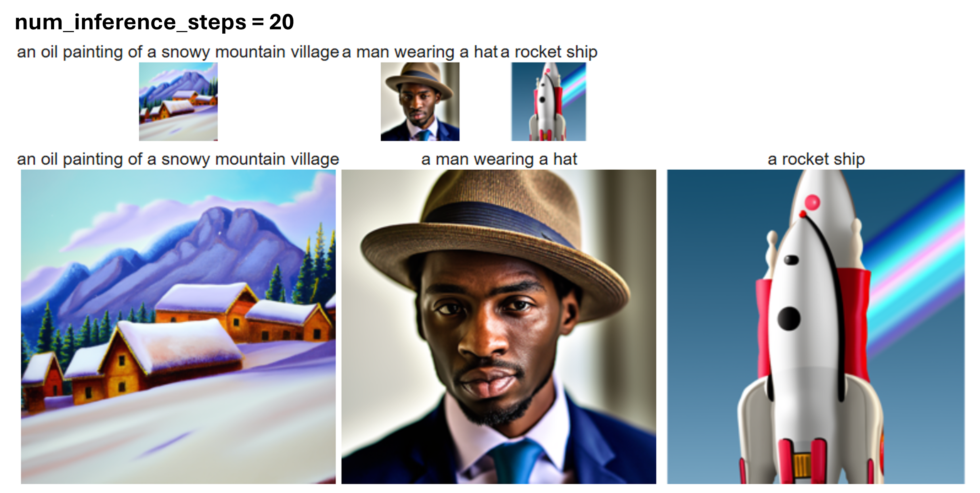
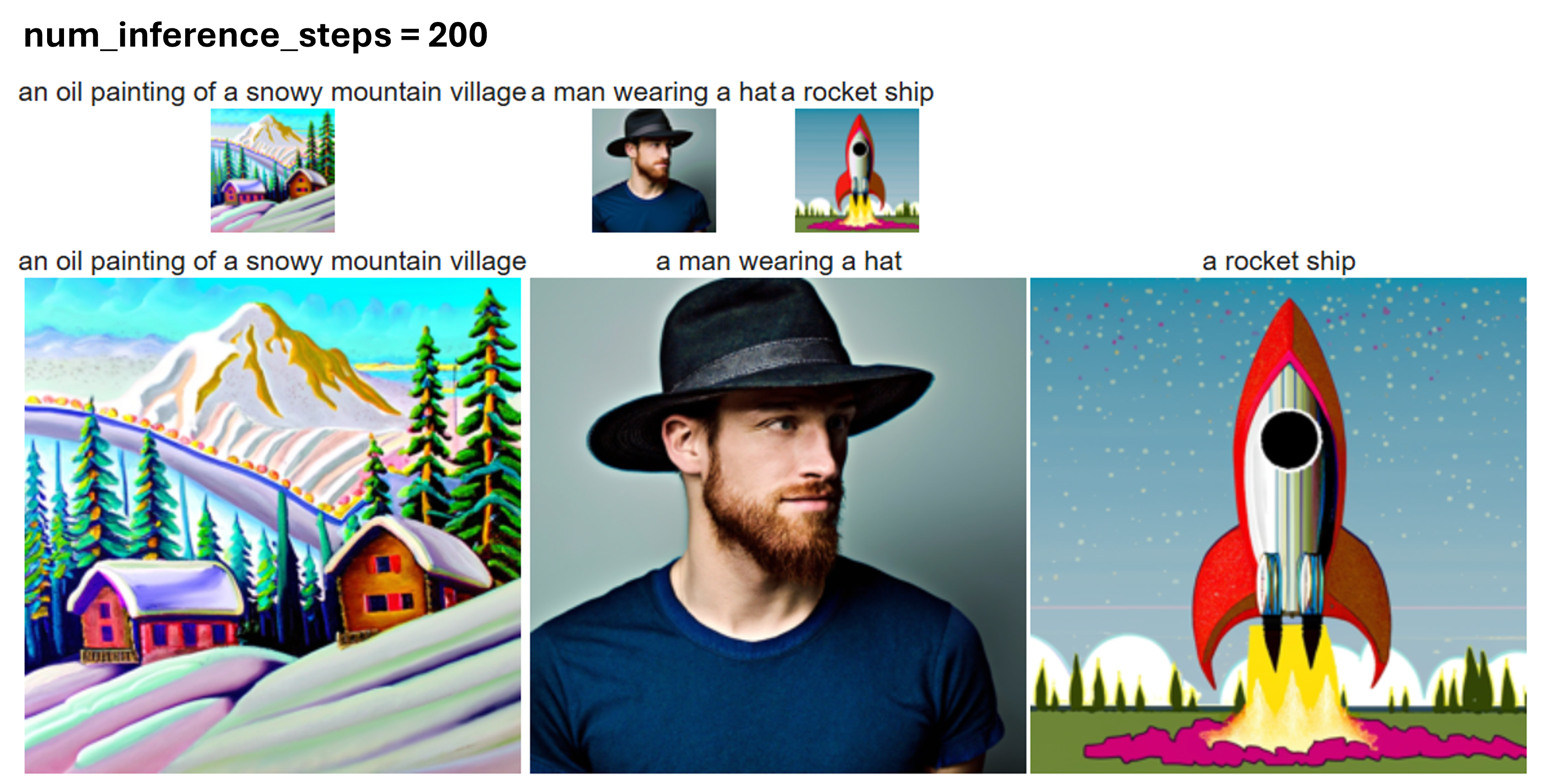
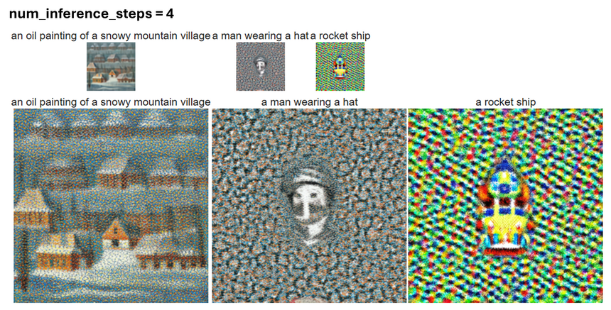
For small num_inference_steps, for example, 5, the output fails to provide sufficient details and contains a lot of noise in the figure. The desciptor from the prompt is poorly reflected in the output. As we increases num_inference_steps, more details are showcased and the output better aligns with the content in the prompt.

Random seed I'm using here is 1998.
num_4
Figure 1: Outputs with num_inference_step = 4.
num_4
Figure 2: Outputs with num_inference_step = 20.
num_4
Figure 3: Outputs with num_inference_step = 200.

Part A.1: Sampling Loops

Part A.1.1: Implementing the Forward Process

A key part of diffusion is the forward process, which takes a clean image and adds noise to it. The forward process is defined by:

$$q(x_t \mid x_0) = \mathcal{N}(x_t; \sqrt{\bar{\alpha}_t}x_0, (1 - \bar{\alpha}_t)\mathbf{I})$$

which is equivalent to computing

$$x_t = \sqrt{\bar{\alpha}_t}x_0 + \sqrt{1 - \bar{\alpha}_t} \epsilon, \quad \text{where } \epsilon \sim \mathcal{N}(0, 1)$$

That is, given a clean image \( x_0 \), we got a noisy image \( x_t \) at timestep \( t \) by sampling from a Gaussian with mean \( \sqrt{\bar{\alpha}_t} x_0 \) and variance \( 1-\bar{\alpha}_t \) Note that the forward process is not just adding the noise - we also scale the image.

In this part, we use the alphas_cumprod variable, which contains the \( \bar{\alpha}_t \) for all \( t \in [0, 999] \). \( t=0 \) corresponds to a clean image and larger \(t\) corresponds to more noise. Thus, \( \bar{\alpha}_t \) is close to 1 for small \( t \), and close to 0 for larger \( t \).

num_4
Figure 4: Test Berkeley Campanile image at noise level [250, 500, 750].

Part A.1.2: Classical Denoising

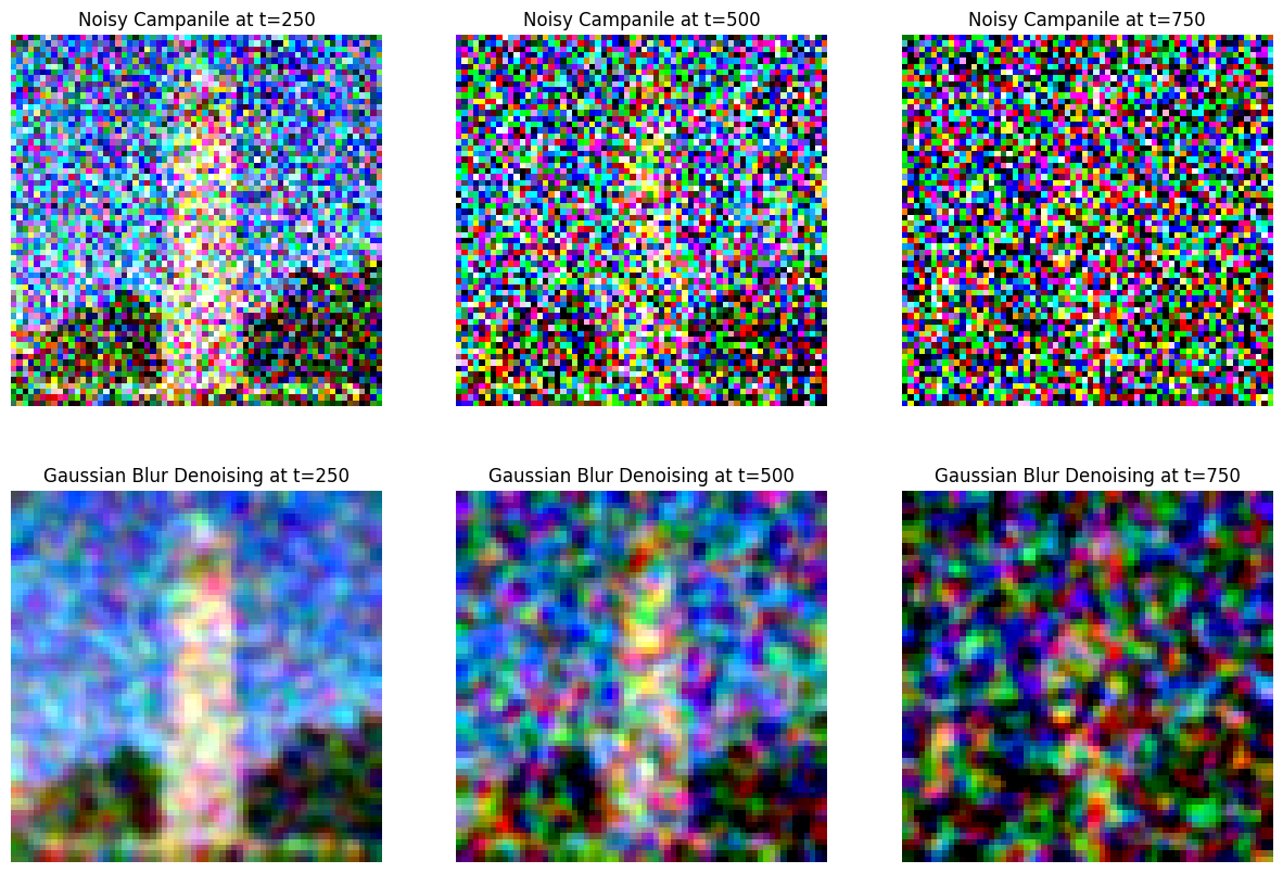
In this part, we take noisy images for timesteps[250, 500, 750], but use Gaussian blur filterring to try to remove noise.

Classic Denoising
Figure 5: Gaussian-denoised version of 3 previous noisy test images.

Part A.1.3: One-Step Denoising

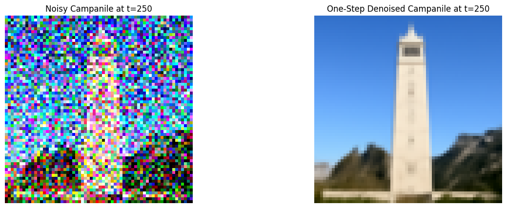
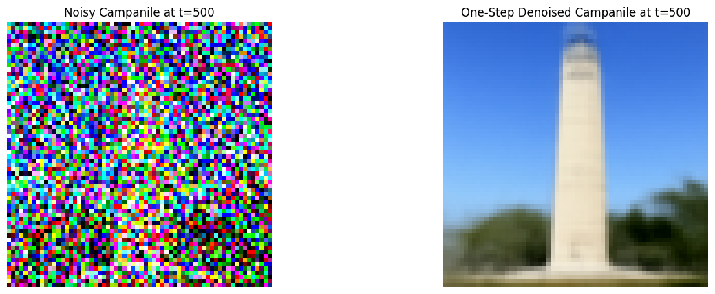
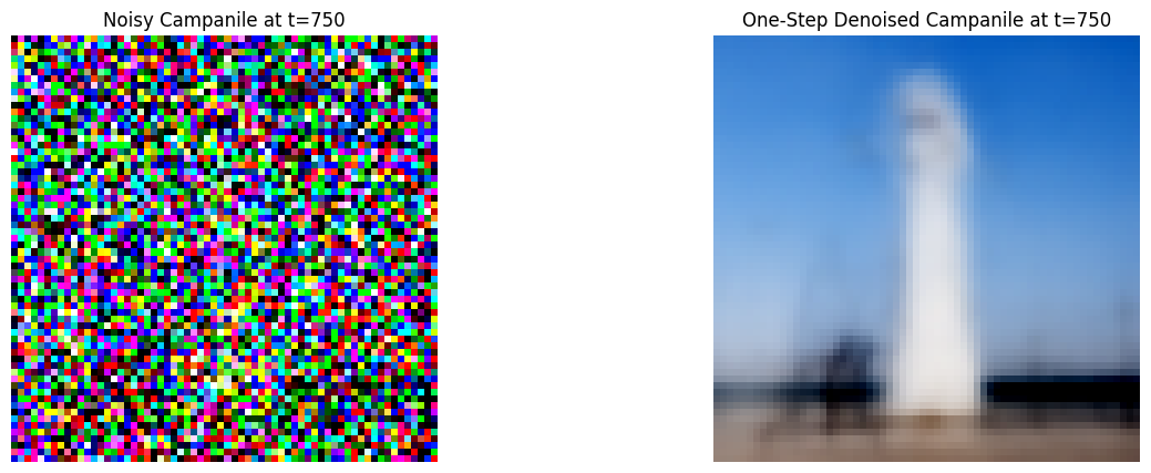
Now, we use a pretrained diffusion model to denoise. The actual denoiser can be found at stage_1.unet. This is a UNet that has already been trained on a very very large dataset of (\(x_0, x_t\)) pairs of images. We can use it to recover Gaussian noise from the image. Then, we can remove this noise to recover (something close to) the original image. The text prompt embedding used here is "a high quality photo".

Classic Denoising
Figure 6-1: Noisy and one-step denoised Campanile at t=250.
Classic Denoising
Figure 6-2: Noisy and one-step denoised Campanile at t=500.
Classic Denoising
Figure 6-3: Noisy and one-step denoised Campanile at t=750.

Part A.1.4: Iterative Denoising

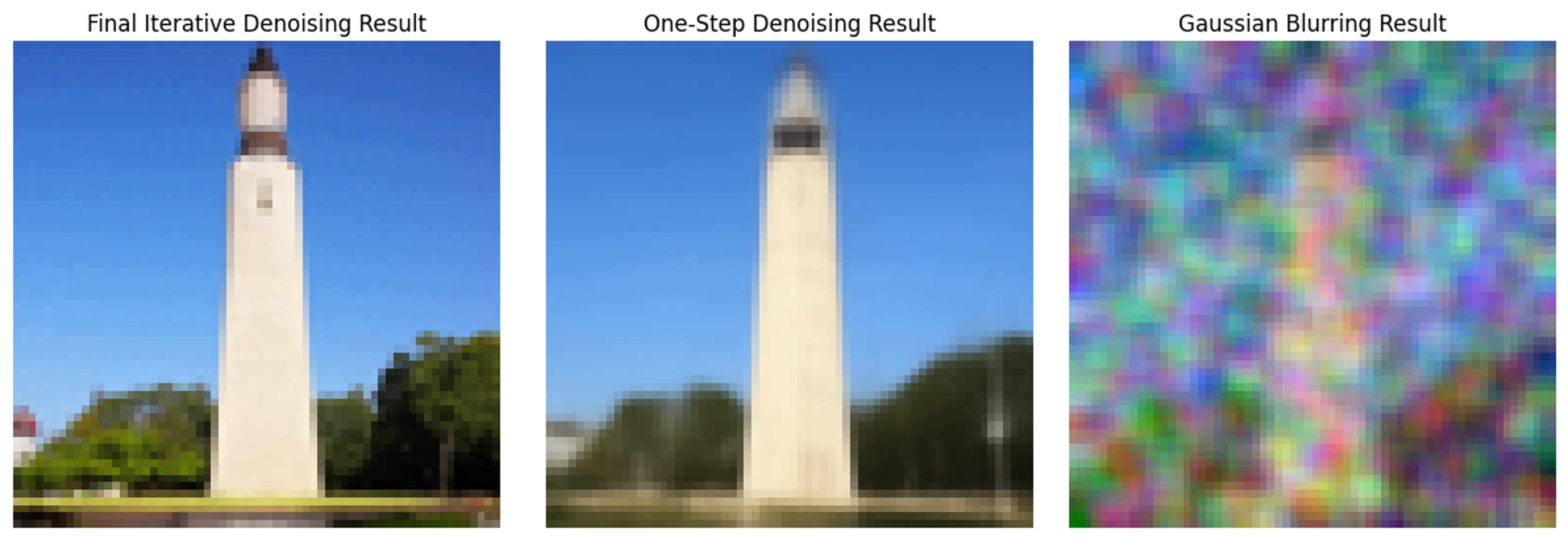
Diffusion models are designed to denoise iteratively.

Iterative Denoising
Figure 7-1: Noisy image every 5th loop of denoising.
Iterative Denoising
Figure 7-2: Final predicted clean image using iterative denoising(left), only a single denoising step(middle) and gaussian blurring(right).

Part A.1.5: Diffusion Model Sampling

Another thing we can do with the iterative_denoise function is to generate images from scratch. We can do this by setting i_start = 0 and passing in random noise. This effectively denoises pure noise. Prompt used here is "a high quality photo".

Iterative Denoising
Figure 8: 5 sampled images.

Part A.1.6: Classifier-Free Guidance (CFG)

In order to greatly improve image quality (at the expense of image diversity), we can use a technique called Classifier-Free Guidance.

In CFG, we compute both a conditional and an conditional noise estimate. We denote these \(\epsilon_c\) and \(\epsilon_u\). Then we let our new noise estimate be:

$$\epsilon = \epsilon_u + \gamma (\epsilon_c - \epsilon_u)$$

where \(\gamma\) controls the strength of CFG. Notice that for \(\gamma=0\), we get an unconditional noise estimate, and for \(\gamma=1\) we get the conditional noise estimate. The magic happens when \(\gamma>1\). In this case, we get much higher quality images.

Classifier-Free Guidance (CFG)
Figure 9: 5 sampled images with CFG.

Part A.1.7: Image-to-image Translation

Here, we run the forward process to get a noisy test image, then run the iterative_denoise_cfg function using a starting index of [1, 3, 5, 7, 10, 20] steps.

Image-to-image Translation
Figure 10-1: SDEdit Berkeley Campanile with i_start = 1,3,5,7,10,20(from left to right).
Image-to-image Translation
Figure 10-2: SDEdit panda with i_start = 1,3,5,7,10,20(from left to right).
Image-to-image Translation
Figure 10-3: SDEdit rose with i_start = 1,3,5,7,10,20(from left to right).

Part A.1.7.1: Editing Hand-Drawn and Web Images

Editing Hand-Drawn and Web Images
Figure 11-1: Web cat image edited using the above method for noise levels [1, 3, 5, 7, 10, 20].
Editing Hand-Drawn and Web Images
Figure 11-2: Hand-drawn cat image edited using the above method for noise levels [1, 3, 5, 7, 10, 20].
Editing Hand-Drawn and Web Images
Figure 11-3: Hand-drawn flower image edited using the above method for noise levels [1, 3, 5, 7, 10, 20].

Part A.1.7.2: Inpainting

We can use the same procedure to implement inpainting. That is, given an image \(x_{orig}\) and a binary mask \(m\), we can create a new image that has the same content where \(m\) is 0, but new content where \(m\) is 1.

Inpainting
Figure 12-1: Inpaint Berkeley Campanile.
Inpainting
Figure 12-2: Inpaint smile emoji(smile:)->shocked:o).
Inpainting
Figure 12-3: Inpaint window (Bear!).

Part A.1.7.3: Text-Conditional Image-to-image Translation

Inpainting
Figure 13-1: Campanile to arocket ship.
Inpainting
Figure 13-1: Dachshund to a pencil.
Inpainting
Figure 13-1: Cat to a photo of a dog.

Part A.1.8: Visual Anagrams

Flipped
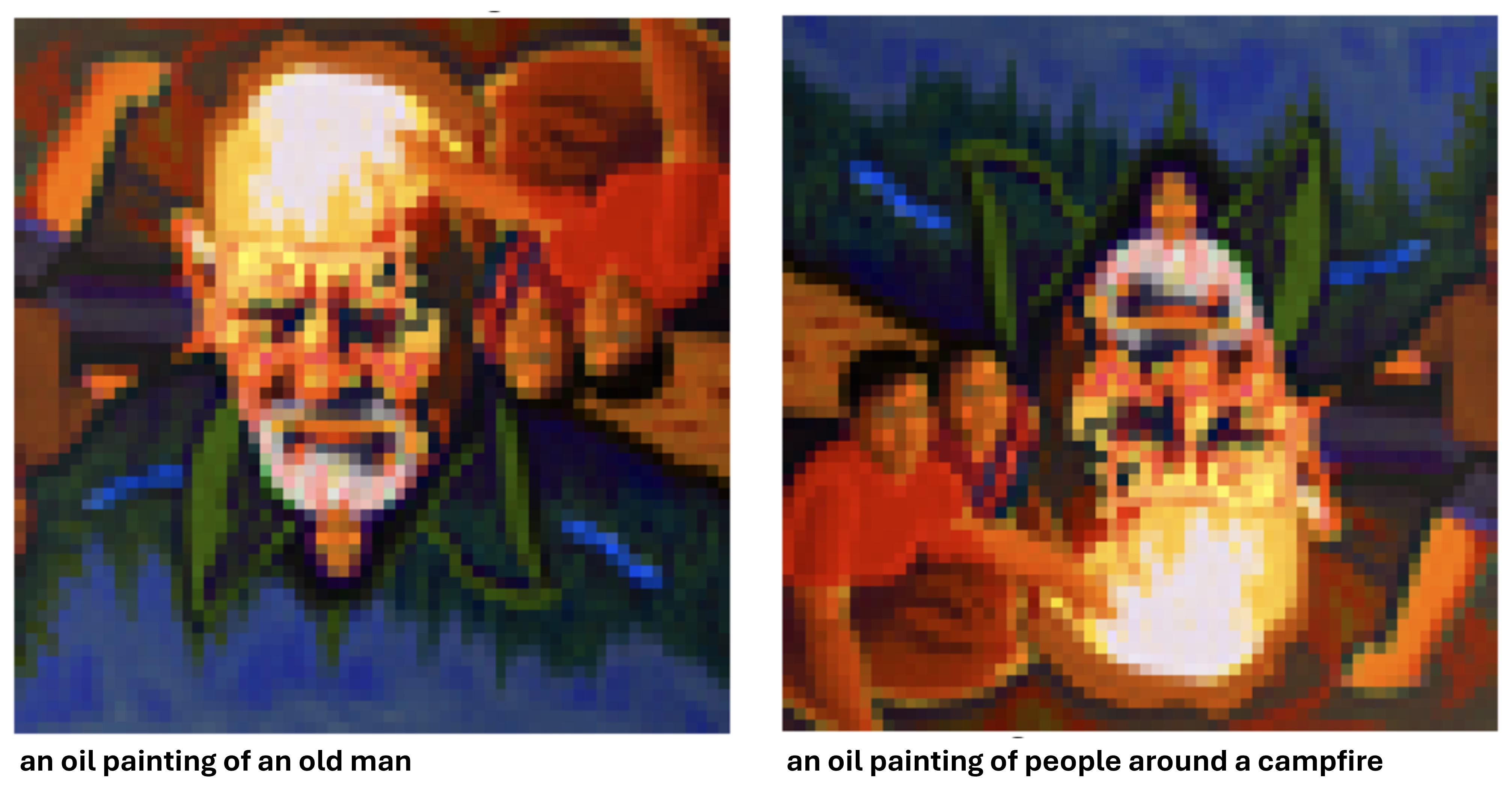
Figure 14-1: Visual anagram where one orientation is "an oil painting of an old man" and when flipped, "an oil painting of people around a campfire".
Flipped
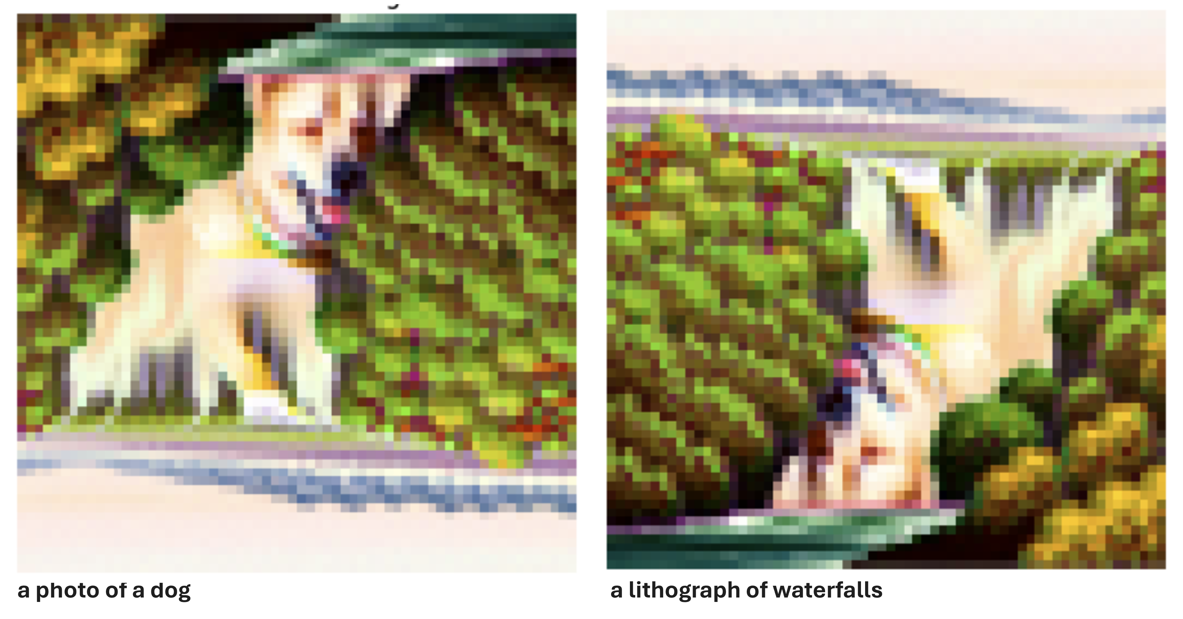
Figure 14-2: Visual anagram where one orientation is "a photo of a dog" and when flipped, "a lithograph of waterfalls".
Flipped
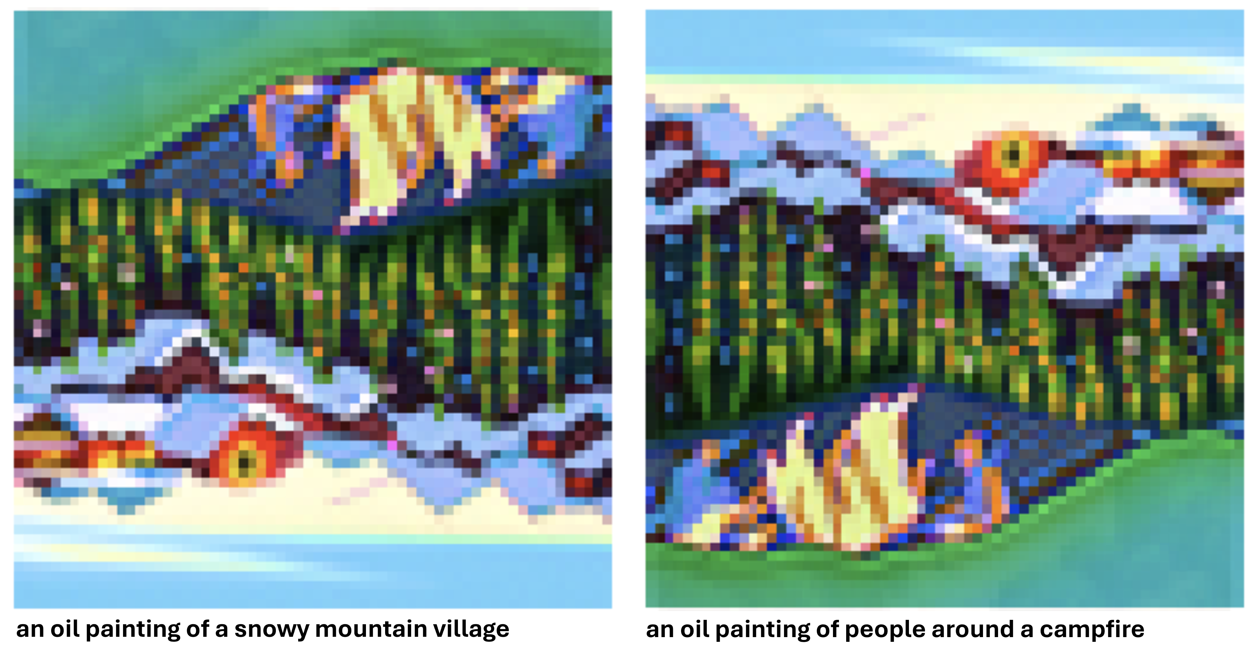
Figure 14-3: Visual anagram where one orientation is "an oil painting of a snowy mountain village" and when flipped, "an oil painting of people around a campfire".

Part A.1.9: Hybrid Images

Hybrid
Figure 15: Hybrid images.

Part B: Diffusion Models from Scratch!

Part B.1: Training a Single-Step Denoising UNet

The first part is to build a simple one-step denoiser. Given a noisy image, we aim to train a denoiser \( D_0 \) such that it maps \( z \) to a clean image \( x \). To do so, we can optimize over an L2 loss:

$$L = \mathbb{E}_{z,x} \| D_\theta(z) - x \|^2$$

Part B.1.1: Implementing the UNet

In this part, we implement the denoiser as a UNet. It consists of a few downsampling and upsampling blocks with skip connections, which uses a number of standard tensor operations.

Unet
Figure 1: Unconditional UNet
Unet
Figure 2: Standard UNet Operations

Part B.1.2 Using the UNet to Train a Denoiser

To train our denoiser, we need to generate training data pairs of (\( z \), \( x \)), where each \( x \) is a clean MNIST digit. For each training batch, we can generate \( z \) from \( x \) using the the following noising process:

$$z = x + \sigma \epsilon, \quad \text{where } \epsilon \sim N(0, I).$$

Visualize the different noising processes over $$\sigma = [0.0, 0.2, 0.4, 0.5, 0.6, 0.8, 1.0]$$assuming normalized $$x \in [0, 1]$$.

Unet
Figure 3: Varying levels of noise on MNIST digits

Part B.1.2.1: Training

Training Loss
Figure 4: Training Loss Curve
Result Epoch 1
Figure 5: Results on digits from the test set after 1 epoch of training
Result Epoch 5
Figure 6: Results on digits from the test set after 5 epoch of training

Part B.1.2.2 Out-of-Distribution Testing

Our denoiser was trained on MNIST digits noised with \( \sigma=0.5 \). Visualize the denoiser results on test set digits with varying levels of noise

$$\sigma = [0.0, 0.2, 0.4, 0.5, 0.6, 0.8, 1.0]$$

varying noise
Figure 7: Results on digits from the test set with varying noise levels

Part B.2: Training a Diffusion Model

Part B.2.1: Adding Time Conditioning to UNet

We need a way to inject scalar \( t \) into our UNet model to condition it.

condition UNet
Figure 8: Conditioned UNet

Part B.2.2: Training the UNet

Basically, we pick a random image from the training set, a random \( t \), and train the denoiser to predict the noise in \( x \). We repeat this for different images and different \( t \) values until the model converges and we are happy.

Algorithm
Figure 9: Algorithm B.1. Training time-conditioned UNet
Training loss
Figure 10: Time-Conditioned UNet training loss curve

Part B.2.3 Sampling from the UNet

Algorithm
Figure 11: Algorithm B.2. Sampling from time-conditioned UNet
Algorithm
Figure 12: Epoch 1
Algorithm
Figure 13: Epoch 5
Algorithm
Figure 14: Epoch 10
Algorithm
Figure 15: Epoch 15
Algorithm
Figure 16: Epoch 20

Part B.2.4: Adding Class-Conditioning to UNet

To make the results better and give us more control for image generation, we can also optionally condition our UNet on the class of the digit 0-9.

Algorithm
Figure 17: Algorithm B.3. Training class-conditioned UNet
Training Loss
Figure 18: Class-conditioned UNet training loss curve

Part B.2.5: Sampling from the Class-Conditioned UNet

The sampling process is the same as part A, where we saw that conditional results aren't good unless we use classifier-free guidance. Use classifier-free guidance with \( \gamma=0.5 \) for this part.et on the class of the digit 0-9.

Algorithm
Figure 19: Algorithm B.4. Sampling from class-conditioned UNet
Training Loss
Figure 20: Epoch 1
Training Loss
Figure 21: Epoch 5
Training Loss
Figure 22: Epoch 10
Training Loss
Figure 23: Epoch 15
Training Loss
Figure 24: Epoch 20